AutoMLSearch for time series problems

In this guide, we’ll show how you can use EvalML to perform an automated search of machine learning pipelines for time series problems. Time series support is still being actively developed in EvalML so expect this page to improve over time.

But first, what is a time series?

A time series is a series of measurements taken at different moments in time (Wikipedia). The main difference between a time series dataset and a normal dataset is that the rows of a time series dataset are ordered with time. This relationship between the rows does not exist in non-time series datasets. In a non-time-series dataset, you can shuffle the rows and the dataset still has the same meaning. If you shuffle the rows of a time series dataset, the relationship between the rows is completely different!

What does AutoMLSearch for time series do?

In a machine learning setting, we are usually interested in using past values of the time series to predict future values. That is what EvalML’s time series functionality is built to do.

Loading the data

In this guide, we work with daily minimum temperature recordings from Melbourne, Austrailia from the beginning of 1981 to end of 1990.

We start by loading the temperature data into two splits. The first split will be a training split consisting of data from 1981 to end of 1989. This is the data we’ll use to find the best pipeline with AutoML. The second split will be a testing split consisting of data from 1990. This is the split we’ll use to evaluate how well our pipeline generalizes on unseen data.

from evalml.demos import load_weather
X, y = load_weather()

train_dates, test_dates = X.Date < "1990-01-01", X.Date >= "1990-01-01"
X_train, y_train = X.ww.loc[train_dates], y.ww.loc[train_dates]
X_test, y_test =  X.ww.loc[test_dates], y.ww.loc[test_dates]

Visualizing the training set

import plotly.graph_objects as go

data = [
    go.Scatter(
        x=X_train["Date"],
        y=y_train,
        mode="lines+markers",
        name="Temperature (C)",
        line=dict(color="#1f77b4"),
    )
]
# Let plotly pick the best date format.
layout = go.Layout(
    title={"text": "Min Daily Temperature, Melbourne 1980-1989"},
    xaxis={"title": "Time"},
    yaxis={"title": "Temperature (C)"},
)

go.Figure(data=data, layout=layout)

Running AutoMLSearch

AutoMLSearch for time series problems works very similarly to the other problem types with the exception that users need to pass in a new parameter called problem_configuration.

The problem_configuration is a dictionary specifying the following values:

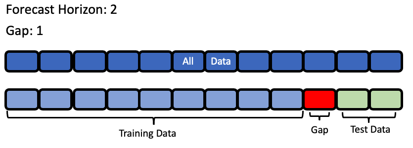
• forecast_horizon: The number of time periods we are trying to forecast. In this example, we’re interested in predicting weather for the next 7 days, so the value is 7.

• gap: The number of time periods between the end of the training set and the start of the test set. For example, in our case we are interested in predicting the weather for the next 7 days with the data as it is “today”, so the gap is 0. However, if we had to predict the weather for next Monday-Sunday with the data as it was on the previous Friday, the gap would be 2 (Saturday and Sunday separate Monday from Friday). It is important to select a value that matches the realistic delay between the forecast date and the most recently avaliable data that can be used to make that forecast.

• max_delay: The maximum number of rows to look in the past from the current row in order to compute features. In our example, we’ll say we can use the previous week’s weather to predict the current week’s.

• date_index: The column of the training dataset that contains the date corresponding to each observation. Currently, this parameter is only used by some time-series specific models so in this example, we are passing in None.

Note that the values of these parameters must be in the same units as the training/testing data.

Visualization of forecast horizon and gap

from evalml.automl import AutoMLSearch

automl = AutoMLSearch(X_train, y_train, problem_type="time series regression",
                      max_batches=1,
                      problem_configuration={"gap": 0, "max_delay": 7,
                                             "forecast_horizon": 7, "date_index": None},
                      allowed_model_families=["xgboost", "random_forest", "linear_model", "extra_trees",
                                              "decision_tree"]
                      )

/home/docs/checkouts/readthedocs.org/user_builds/feature-labs-inc-evalml/envs/v0.35.0/lib/python3.8/site-packages/evalml/automl/automl_search.py:456: UserWarning:

Time series support in evalml is still in beta, which means we are still actively building its core features. Please be mindful of that when running search().

automl.search()

/home/docs/checkouts/readthedocs.org/user_builds/feature-labs-inc-evalml/envs/v0.35.0/lib/python3.8/site-packages/sklearn/linear_model/_coordinate_descent.py:530: ConvergenceWarning:

Objective did not converge. You might want to increase the number of iterations. Duality gap: 4089.24423870312, tolerance: 1.7012860284653468

/home/docs/checkouts/readthedocs.org/user_builds/feature-labs-inc-evalml/envs/v0.35.0/lib/python3.8/site-packages/sklearn/linear_model/_coordinate_descent.py:530: ConvergenceWarning:

Objective did not converge. You might want to increase the number of iterations. Duality gap: 7638.417351298465, tolerance: 2.9630934475138115

/home/docs/checkouts/readthedocs.org/user_builds/feature-labs-inc-evalml/envs/v0.35.0/lib/python3.8/site-packages/sklearn/linear_model/_coordinate_descent.py:530: ConvergenceWarning:

Objective did not converge. You might want to increase the number of iterations. Duality gap: 11061.119581322855, tolerance: 4.09238672

Understanding what happened under the hood

This is great, AutoMLSearch is able to find a pipeline that scores an R2 value of 0.44 compared to a baseline pipeline that is only able to score 0.07. But how did it do that?

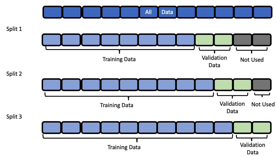
Data Splitting

EvalML uses rolling origin cross validation for time series problems. Basically, we take successive cuts of the training data while keeping the validation set size fixed. Note that the splits are not separated by gap number of units. This is because we need access to all the data to generate features for every row of the validation set. However, the feature engineering done by our pipelines respects the gap value. This is explained more in the feature engineering section.

Baseline Pipeline

The most naive thing we can do in a time series problem is use the most recently available observation to predict the next observation. In our example, this means we’ll use the measurement from 7 days ago as the prediction for the current date.

import pandas as pd
baseline = automl.get_pipeline(0)
baseline.fit(X_train, y_train)
naive_baseline_preds = baseline.predict_in_sample(X_test, y_test, objective=None,
                                                  X_train=X_train, y_train=y_train)
expected_preds = pd.concat([y_train.iloc[-7:], y_test]).shift(7).iloc[7:]
pd.testing.assert_series_equal(expected_preds, naive_baseline_preds)

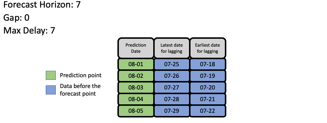
Feature Engineering

EvalML uses the values of gap, forecast_horizon, and max_delay to calculate a “window” of allowed dates that can be used for engineering the features of each row in the validation/test set. The formula for computing the bounds of the window is:

[t - (max_delay + forecast_horizon + gap), t - (forecast_horizon + gap)]

As an example, this is what the features for the first five days of August would look like in our current problem:

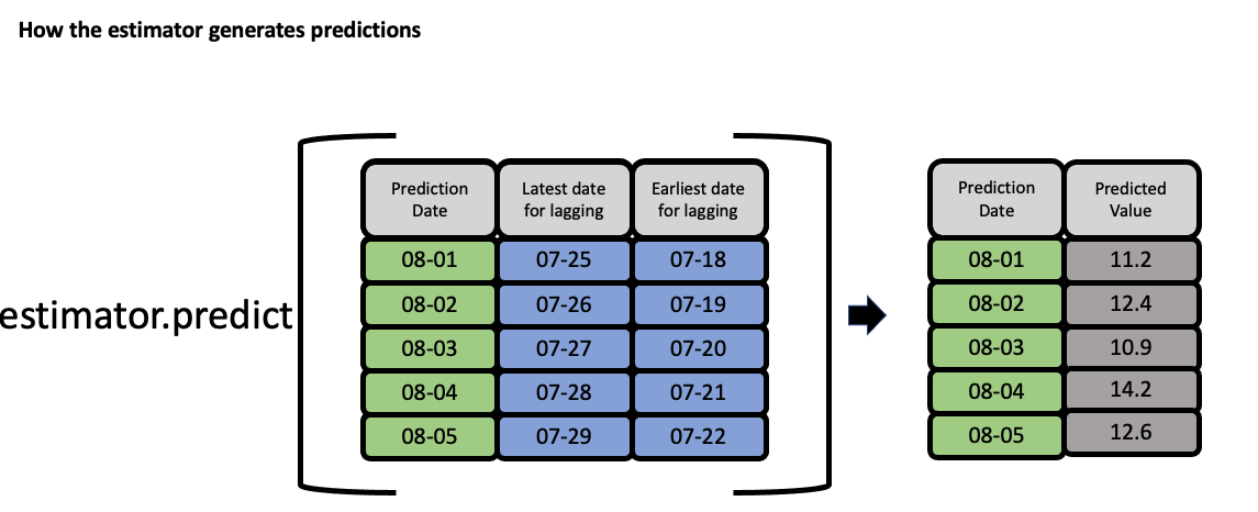
The estimator then takes these features to generate predictions:

Evaluate best pipeline on test data

Now that we have covered the mechanics of how EvalML runs AutoMLSearch for time series pipelines, we can compare the performance on the test set of the best pipeline found during search and the baseline pipeline.

pl = automl.best_pipeline

pl.fit(X_train, y_train)

best_pipeline_score = pl.score(X_test, y_test, ['R2'], X_train, y_train)['R2']

best_pipeline_score

0.5502791890460579

baseline = automl.get_pipeline(0)
baseline.fit(X_train, y_train)
naive_baseline_score = baseline.score(X_test, y_test, ['R2'], X_train, y_train)['R2']

naive_baseline_score

0.14924457197371788

The pipeline found by AutoMLSearch has a 268% improvement over the naive forecast!

automl.objective.calculate_percent_difference(best_pipeline_score, naive_baseline_score)

268.7096835541615

Visualize the predictions over time

from evalml.model_understanding import graph_prediction_vs_actual_over_time

fig = graph_prediction_vs_actual_over_time(pl, X_test, y_test, X_train, y_train, dates=X_test['Date'])
fig

Predicting on unseen data

You’ll notice that in the code snippets here, we use the predict_in_sample pipeline method as opposed to the usual predict method. What’s the difference?

• predict_in_sample is used when the target value is known on the dates we are predicting on. This is true in cross validation. This method has an expected y parameter so that we can compute features using previous target values for all of the observations on the holdout set.

• predict is used when the target value is not known, e.g. the test dataset. The y parameter is not expected as only the target is observed in the training set. The test dataset must be separated by gap days from the training dataset. For the moment, the test set size must match forecast_horizon.

Here is an example of these two methods in action:

predict_in_sample

pl.predict_in_sample(X_test, y_test, objective=None, X_train=X_train, y_train=y_train)

3285    14.222870
3286    14.278846
3287    14.022847
3288    13.738781
3289    13.530056
          ...
3645    14.148007
3646    13.927396
3647    14.022316
3648    14.045560
3649    13.694097
Name: Temp, Length: 365, dtype: float64

predict

pl.predict(X_test.iloc[:pl.forecast_horizon], objective=None, X_train=X_train, y_train=y_train)

3285    14.222870
3286    14.278846
3287    14.022847
3288    13.738781
3289    13.530056
3290    13.988278
3291    13.638807
Name: Temp, dtype: float64

previous

Utilities

next

FAQ