AutoMLSearch for time series problems

In this guide, we’ll show how you can use EvalML to perform an automated search of machine learning pipelines for time series problems. Time series support is still being actively developed in EvalML so expect this page to improve over time.

But first, what is a time series?

A time series is a series of measurements taken at different moments in time (Wikipedia). The main difference between a time series dataset and a normal dataset is that the rows of a time series dataset are ordered chronologically, where the relative time between rows is significant. This relationship between the rows does not exist in non-time series datasets. In a non-time-series dataset, you can shuffle the rows and the dataset still has the same meaning. If you shuffle the rows of a time series dataset, the relationship between the rows is completely different!

What does AutoMLSearch for time series do?

In a machine learning setting, we are usually interested in using past values of the time series to predict future values. That is what EvalML’s time series functionality is built to do.

Loading the data

In this guide, we work with daily minimum temperature recordings from Melbourne, Austrailia from the beginning of 1981 to end of 1990.

We start by loading the temperature data into two splits. The first split will be a training split consisting of data from 1981 to end of 1989. This is the data we’ll use to find the best pipeline with AutoML. The second split will be a testing split consisting of data from 1990. This is the split we’ll use to evaluate how well our pipeline generalizes on unseen data.

import pandas as pd
from evalml.demos import load_weather

X, y = load_weather()

             Number of Features
Categorical                   1

Number of training examples: 3650
Targets
10.0    1.40%
11.0    1.40%
13.0    1.32%
12.5    1.21%
10.5    1.21%
        ...
0.2     0.03%
24.0    0.03%
25.2    0.03%
22.7    0.03%
21.6    0.03%
Name: Temp, Length: 229, dtype: object

train_dates, test_dates = X.Date < "1990-01-01", X.Date >= "1990-01-01"
X_train, y_train = X.ww.loc[train_dates], y.ww.loc[train_dates]
X_test, y_test = X.ww.loc[test_dates], y.ww.loc[test_dates]

Visualizing the training set

import plotly.graph_objects as go

data = [
    go.Scatter(
        x=X_train["Date"],
        y=y_train,
        mode="lines+markers",
        name="Temperature (C)",
        line=dict(color="#1f77b4"),
    )
]
# Let plotly pick the best date format.
layout = go.Layout(
    title={"text": "Min Daily Temperature, Melbourne 1980-1989"},
    xaxis={"title": "Time"},
    yaxis={"title": "Temperature (C)"},
)

go.Figure(data=data, layout=layout)

Fixing the data

Sometimes, the datasets we work with do not have perfectly consistent DateTime columns. We can use the TimeSeriesRegularizer and TimeSeriesImputer to correct any discrepancies in our data in a time-series specific way.

To show an example of this, let’s create some discrepancies in our training data. We’ll also add a couple of extra columns in the X DataFrame to highlight more of the options with these tools.

X["Categorical"] = [str(i % 4) for i in range(len(X))]
X["Numeric"] = [i for i in range(len(X))]

# Re-split the data since we modified X
X_train, y_train = X.loc[train_dates], y.ww.loc[train_dates]
X_test, y_test = X.loc[test_dates], y.ww.loc[test_dates]

X_train["Date"][500] = None
X_train["Date"][1042] = None
X_train["Date"][1043] = None
X_train["Date"][231] = pd.Timestamp("1981-08-19")

X_train.drop(1209, inplace=True)
X_train.drop(398, inplace=True)
y_train.drop(1209, inplace=True)
y_train.drop(398, inplace=True)

With these changes, there are now NaN values in the training data that our models won’t be able to recognize, and there is no longer a clear frequency between the dates.

print(f"Inferred frequency: {pd.infer_freq(X_train['Date'])}")
print(f"NaNs in date column: {X_train['Date'].isna().any()}")
print(
    f"NaNs in other training data columns: {X_train['Categorical'].isna().any() or X_train['Numeric'].isna().any()}"
)
print(f"NaNs in target data: {y_train.isna().any()}")

Inferred frequency: None
NaNs in date column: True
NaNs in other training data columns: False
NaNs in target data: False

Time Series Regularizer

We can use the TimeSeriesRegularizer component to restore the missing and NaN DateTime values we’ve created in our data. This component is designed to infer the proper frequency using Woodwork’s “infer_frequency” function and generate a new DataFrame that follows it. In order to maintain as much original information from the input data as possible, all rows with completely correct times are ported over into this new DataFrame. If there are any rows that have the same timestamp as another, these will be dropped. The first occurrence of a date or time maintains priority. If there are any values that don’t quite line up with the inferred frequency they will be shifted to any closely missing datetimes, or dropped if there are none nearby.

from evalml.pipelines.components import TimeSeriesRegularizer

regularizer = TimeSeriesRegularizer(time_index="Date")
X_train, y_train = regularizer.fit_transform(X_train, y_train)

Now we can see that pandas has successfully inferred the frequency of the training data, and there are no more null values within X_train. However, by adding values that were dropped before, we have created NaN values within the target data, as well as the other columns in our training data.

print(f"Inferred frequency: {pd.infer_freq(X_train['Date'])}")
print(f"NaNs in training data: {X_train['Date'].isna().any()}")
print(
    f"NaNs in other training data columns: {X_train['Categorical'].isna().any() or X_train['Numeric'].isna().any()}"
)
print(f"NaNs in target data: {y_train.isna().any()}")

Inferred frequency: D
NaNs in training data: False
NaNs in other training data columns: True
NaNs in target data: True

Time Series Imputer

We could easily use the Imputer and TargetImputer components to fill in the missing gaps in our X and y data. However, these tools are not built for time series problems. Their supported imputation strategies of “mean”, “most_frequent”, or similar are all static. They don’t account for the passing of time, and how neighboring data points may have more predictive power than simply taking the average. The TimeSeriesImputer solves this problem by offering three different imputation strategies: - “forwards_fill”: fills in any NaN values with the same value as found in the previous non-NaN cell. - “backwards_fill”: fills in any NaN values with the same value as found in the next non-NaN cell. - “interpolate”: (numeric columns only) fills in any NaN values by linearly interpolating the values of the previous and next non-NaN cells.

from evalml.pipelines.components import TimeSeriesImputer

ts_imputer = TimeSeriesImputer(
    categorical_impute_strategy="forwards_fill",
    numeric_impute_strategy="backwards_fill",
    target_impute_strategy="interpolate",
)
X_train, y_train = ts_imputer.fit_transform(X_train, y_train)

Now, finally, we have a DataFrame that’s back in order without flaws, which we can use for running AutoMLSearch and running models without issue.

print(f"Inferred frequency: {pd.infer_freq(X_train['Date'])}")
print(f"NaNs in training data: {X_train['Date'].isna().any()}")
print(
    f"NaNs in other training data columns: {X_train['Categorical'].isna().any() or X_train['Numeric'].isna().any()}"
)
print(f"NaNs in target data: {y_train.isna().any()}")

Inferred frequency: D
NaNs in training data: False
NaNs in other training data columns: False
NaNs in target data: False

Trending and Seasonality Decomposition

Decomposing a target signal into a trend and/or a cyclical signal is a common pre-processing step for time series modeling. Having an understanding of the presence or absence of these component signals can provide additional insight and decomposing the signal into these constituent components can enable non-time-series aware estimators to perform better while attempting to model this data. We have two unique decomposers, the PolynomialDecompser and the STLDecomposer.

Let’s first take a look at a year’s worth of the weather dataset.

import matplotlib.pyplot as plt

length = 365
X_train_time = X_train.set_index("Date").asfreq(pd.infer_freq(X_train["Date"]))
y_train_time = y_train.set_axis(X_train["Date"]).asfreq(pd.infer_freq(X_train["Date"]))
plt.plot(y_train_time[0:length], "bo")
plt.show()

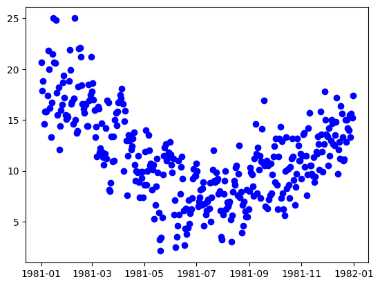
With the knowledge that this is a weather dataset and the data itself is daily weather data, we can assume that the seasonal data will have a period of approximately 365 data points. Let’s build and fit decomposers to detrend and deseasonalize this data.

Polynomial Decomposer

from evalml.pipelines.components.transformers.preprocessing.polynomial_decomposer import (
    PolynomialDecomposer,
)

pdc = PolynomialDecomposer(degree=1, period=365)
X_t, y_t = pdc.fit_transform(X_train_time, y_train_time)

plt.plot(y_train_time, "bo", label="Signal")
plt.plot(y_t, "rx", label="Detrended/Deseasonalized Signal")
plt.legend()
plt.show()

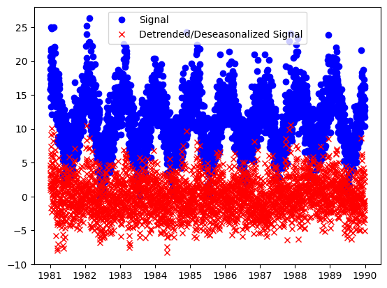
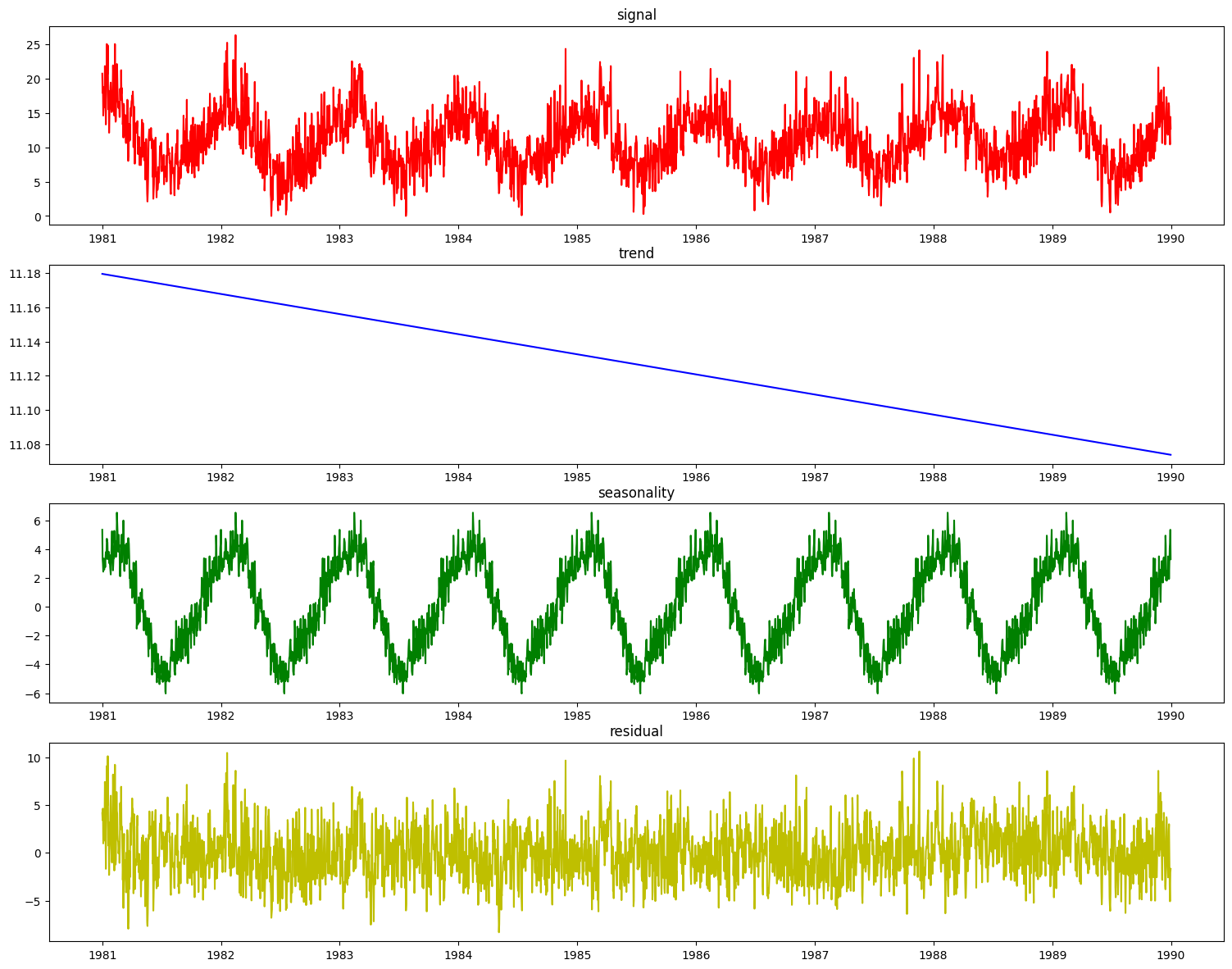
The result is the residual signal, with the trend and seasonality removed. If we want to look at what the component identified as the trend and seasonality, we can call the plot_decomposition() function.

res = pdc.plot_decomposition(X_train_time, y_train_time)

It is desirable to enhance the decomposer component with a guess at the period of the seasonal aspect of the signal before decomposing it. To do that, we can use the determine_periodicity(X, y) function of the Decomposer class.

period = pdc.determine_periodicity(X_train_time, y_train_time)
print(period)

351

The PolynomialDecomposer class, if not explicitly set in the constructor, will set its period parameter based on a statsmodels function freq_to_period that considers the frequency of the datetime data. This will give a reasonable guess as to what the frequency could be. For example, if the PolynomialDecomposer object is fit with period not explicitly set, it will take on a default value of 7, which is good for daily data signals that have a known seasonal component period that is weekly.

In this case where the seasonal period is not known beforehand, the set_period() convenience function will look at the target data, determine a better guess for the period and set the Decomposer object appropriately.

pdc = PolynomialDecomposer()
pdc.fit(X_train_time, y_train_time)
assert pdc.period == 7
pdc.set_period(X_train_time, y_train_time)
assert 350 < pdc.period < 370

STLDecomposer

The STLDecomposer runs on statsmodels’ implementation of STL decomposition. Let’s take a look at how STL decomposes the weather dataset.

from evalml.pipelines.components import STLDecomposer

stl = STLDecomposer()
X_t, y_t = stl.fit_transform(X_train_time, y_train_time)

res = stl.plot_decomposition(X_train_time, y_train_time)

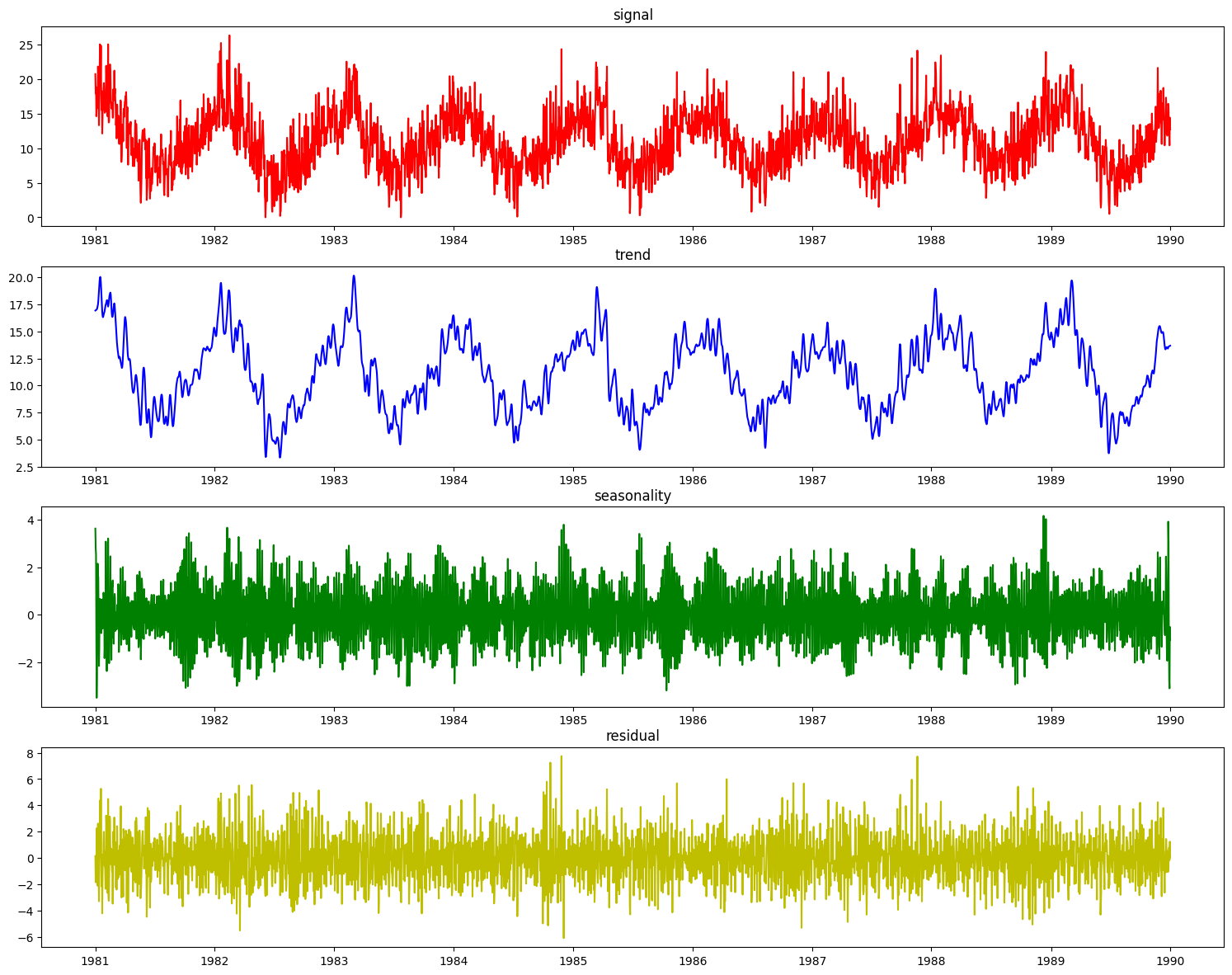
This doesn’t look nearly as good as the PolynomialDecomposer did. This is because STL decomposition performs best when the data has a small seasonal period, generally less than 14 time units. The weather dataset’s seasonal period of ~365 days does not work as well since STL extracted a shorter term seasonality for decomposition.

We can generate some synthetic data that better highlights where STL performs well. For this example, we’ll generate monthly data with an annual seasonal period.

import random
import numpy as np
from datetime import datetime
from sklearn.preprocessing import minmax_scale


def generate_synthetic_data(
    period=12,
    num_periods=25,
    scale=10,
    seasonal_scale=2,
    trend_degree=1,
    freq_str="M",
):
    freq = 2 * np.pi / period
    x = np.arange(0, period * num_periods, 1)
    dts = pd.date_range(datetime.today(), periods=len(x), freq=freq_str)
    X = pd.DataFrame({"x": x})
    X = X.set_index(dts)

    if trend_degree == 1:
        y_trend = pd.Series(scale * minmax_scale(x + 2))
    elif trend_degree == 2:
        y_trend = pd.Series(scale * minmax_scale(x**2))
    elif trend_degree == 3:
        y_trend = pd.Series(scale * minmax_scale((x - 5) ** 3 + x**2))
    y_seasonal = pd.Series(seasonal_scale * np.sin(freq * x))
    y_random = pd.Series(np.random.normal(0, 1, len(X)))
    y = y_trend + y_seasonal + y_random
    return X, y


X_stl, y_stl = generate_synthetic_data()

Let’s see how the STLDecomposer does at decomposing this data.

stl = STLDecomposer()
X_t_stl, y_t_stl = stl.fit_transform(X_stl, y_stl)

res = stl.plot_decomposition(X_stl, y_stl)

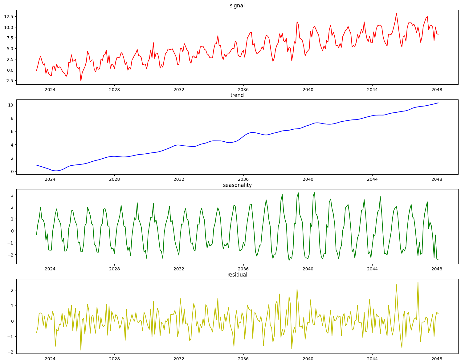
On top of decomposing this type of data well, the statsmodels implementation of STL automatically determines the seasonal period of the data, which is saved during fit time for this component.

stl = STLDecomposer()
assert stl.period == None
stl.fit(X_stl, y_stl)
print(stl.period)

12

Running AutoMLSearch

AutoMLSearch for time series problems works very similarly to the other problem types with the exception that users need to pass in a new parameter called problem_configuration.

The problem_configuration is a dictionary specifying the following values:

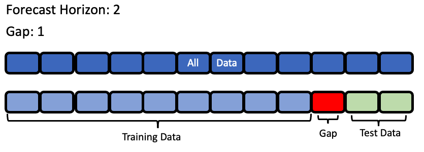
• forecast_horizon: The number of time periods we are trying to forecast. In this example, we’re interested in predicting weather for the next 7 days, so the value is 7.

• gap: The number of time periods between the end of the training set and the start of the test set. For example, in our case we are interested in predicting the weather for the next 7 days with the data as it is “today”, so the gap is 0. However, if we had to predict the weather for next Monday-Sunday with the data as it was on the previous Friday, the gap would be 2 (Saturday and Sunday separate Monday from Friday). It is important to select a value that matches the realistic delay between the forecast date and the most recently avaliable data that can be used to make that forecast.

• max_delay: The maximum number of rows to look in the past from the current row in order to compute features. In our example, we’ll say we can use the previous week’s weather to predict the current week’s.

• time_index: The column of the training dataset that contains the date corresponding to each observation. While only some of the models we run during time series searches require the time_index, we require it to be passed in to top level search so that the parameter can reach the models that need it.

Note that the values of these parameters must be in the same units as the training/testing data.

Visualization of forecast horizon and gap

from evalml.automl import AutoMLSearch

problem_config = {"gap": 0, "max_delay": 7, "forecast_horizon": 7, "time_index": "Date"}

automl = AutoMLSearch(
    X_train,
    y_train,
    problem_type="time series regression",
    max_batches=1,
    problem_configuration=problem_config,
    allowed_model_families=[
        "xgboost",
        "random_forest",
        "linear_model",
        "extra_trees",
        "decision_tree",
    ],
)

/home/docs/checkouts/readthedocs.org/user_builds/feature-labs-inc-evalml/envs/v0.67.0/lib/python3.8/site-packages/evalml/automl/automl_search.py:519: UserWarning:

Time series support in evalml is still in beta, which means we are still actively building its core features. Please be mindful of that when running search().

automl.search()

{1: {'Elastic Net Regressor w/ Replace Nullable Types Transformer + Imputer + Time Series Featurizer + STL Decomposer + DateTime Featurizer + One Hot Encoder + Drop NaN Rows Transformer + Standard Scaler': '00:05',
  'Random Forest Regressor w/ Replace Nullable Types Transformer + Imputer + Time Series Featurizer + STL Decomposer + DateTime Featurizer + One Hot Encoder + Drop NaN Rows Transformer': '00:07',
  'Elastic Net Regressor w/ Replace Nullable Types Transformer + Imputer + Time Series Featurizer + DateTime Featurizer + One Hot Encoder + Drop NaN Rows Transformer + Standard Scaler': '00:03',
  'Random Forest Regressor w/ Replace Nullable Types Transformer + Imputer + Time Series Featurizer + DateTime Featurizer + One Hot Encoder + Drop NaN Rows Transformer': '00:05',
  'Total time of batch': '00:21'}}

Understanding what happened under the hood

This is great, AutoMLSearch is able to find a pipeline that scores an R2 value of 0.44 compared to a baseline pipeline that is only able to score 0.07. But how did it do that?

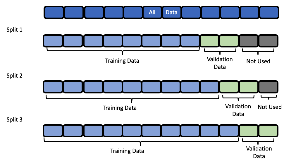
Data Splitting

EvalML uses rolling origin cross validation for time series problems. Basically, we take successive cuts of the training data while keeping the validation set size fixed at forecast_horizon number of time units. Note that the splits are not separated by gap number of units. This is because we need access to all the data to generate features for every row of the validation set. However, the feature engineering done by our pipelines respects the gap value. This is explained more in the feature engineering section.

Baseline Pipeline

The most naive thing we can do in a time series problem is use the most recently available observation to predict the next observation. In our example, this means we’ll use the measurement from 7 days ago as the prediction for the current date.

import pandas as pd

baseline = automl.get_pipeline(0)
baseline.fit(X_train, y_train)
naive_baseline_preds = baseline.predict_in_sample(
    X_test, y_test, objective=None, X_train=X_train, y_train=y_train
)
expected_preds = pd.Series(
    pd.concat([y_train.iloc[-7:], y_test]).shift(7).iloc[7:], name="target"
)
pd.testing.assert_series_equal(expected_preds, naive_baseline_preds)

Feature Engineering

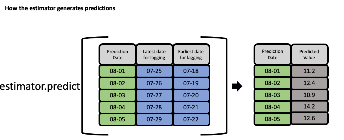
EvalML uses the values of gap, forecast_horizon, and max_delay to calculate a “window” of allowed dates that can be used for engineering the features of each row in the validation/test set. The formula for computing the bounds of the window is:

[t - (max_delay + forecast_horizon + gap), t - (forecast_horizon + gap)]

As an example, this is what the features for the first five days of August would look like in our current problem:

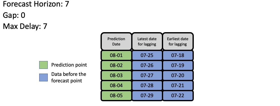
The estimator then takes these features to generate predictions:

Feature engineering components for time series

For an example of a time-series feature engineering component see TimeSeriesFeaturizer

Evaluate best pipeline on test data

Now that we have covered the mechanics of how EvalML runs AutoMLSearch for time series pipelines, we can compare the performance on the test set of the best pipeline found during search and the baseline pipeline.

pl = automl.best_pipeline

pl.fit(X_train, y_train)

best_pipeline_score = pl.score(X_test, y_test, ["MedianAE"], X_train, y_train)[
    "MedianAE"
]

best_pipeline_score

1.8867196350647752

baseline = automl.get_pipeline(0)
baseline.fit(X_train, y_train)
naive_baseline_score = baseline.score(X_test, y_test, ["MedianAE"], X_train, y_train)[
    "MedianAE"
]

naive_baseline_score

2.3

The pipeline found by AutoMLSearch has a 31% improvement over the naive forecast!

automl.objective.calculate_percent_difference(best_pipeline_score, naive_baseline_score)

17.96871151892281

Visualize the predictions over time

from evalml.model_understanding import graph_prediction_vs_actual_over_time

fig = graph_prediction_vs_actual_over_time(
    pl, X_test, y_test, X_train, y_train, dates=X_test["Date"]
)
fig

Predicting on unseen data

You’ll notice that in the code snippets here, we use the predict_in_sample pipeline method as opposed to the usual predict method. What’s the difference?

• predict_in_sample is used when the target value is known on the dates we are predicting on. This is true in cross validation. This method has an expected y parameter so that we can compute features using previous target values for all of the observations on the holdout set.

• predict is used when the target value is not known, e.g. the test dataset. The y parameter is not expected as only the target is observed in the training set. The test dataset must be separated by gap units from the training dataset. For the moment, the test set size must be less than or equal to forecast_horizon.

Here is an example of these two methods in action:

predict_in_sample

pl.predict_in_sample(X_test, y_test, objective=None, X_train=X_train, y_train=y_train)

3287    13.124784
3288    13.468004
3289    13.472009
3290    12.724985
3291    11.868053
          ...
3647    14.159499
3648    13.257666
3649    13.365598
3650    13.731870
3651    12.263210
Name: target, Length: 365, dtype: float64

predict

pl.predict(X_test, objective=None, X_train=X_train, y_train=y_train)

3287    13.124784
3288    13.468004
3289    13.472009
3290    12.724985
3291    11.868053
          ...
3647    18.339399
3648    18.393293
3649    18.464086
3650    18.354281
3651    18.330683
Name: target, Length: 365, dtype: float64

Validating the holdout data

Before we predict on our holdout data, it is important to validate that it meets the requirements we summarized in the second point above in Predicting on unseen data. We can call on validate_holdout_datasets in order to verify the two requirements:

1. The holdout data is separated by gap units from the training dataset. This is determined by the time_index column, not the index e.g. if your datetime frequency for the column “Date” is 2 days with a gap of 3, then the holdout data must start 2 days x 3 = 6 days after the training data.

2. The length of the holdout data must be less than or equal to the forecast_horizon.

from evalml.utils.gen_utils import validate_holdout_datasets

# Holdout dataset has 365 observations
validation_results = validate_holdout_datasets(X_test, X_train, problem_config)
assert not validation_results.is_valid
# Holdout dataset has 7 observations
validation_results = validate_holdout_datasets(
    X_test.iloc[: pl.forecast_horizon], X_train, problem_config
)
assert validation_results.is_valid

predict – Test set size matches forecast horizon

pl.predict(
    X_test.iloc[: pl.forecast_horizon], objective=None, X_train=X_train, y_train=y_train
)

3287    13.124784
3288    13.468004
3289    13.472009
3290    12.724985
3291    11.868053
3292    13.315326
3293    12.943245
Name: target, dtype: float64

predict – Test set size is less than forecast horizon

pl.predict(
    X_test.iloc[: pl.forecast_horizon - 2],
    objective=None,
    X_train=X_train,
    y_train=y_train,
)

3287    13.124784
3288    13.468004
3289    13.472009
3290    12.724985
3291    11.868053
Name: target, dtype: float64

predict – Test set size index starts at 0

pl.predict(
    X_test.iloc[: pl.forecast_horizon].reset_index(drop=True),
    objective=None,
    X_train=X_train,
    y_train=y_train,
)

3287    13.124784
3288    13.468004
3289    13.472009
3290    12.724985
3291    11.868053
3292    13.315326
3293    12.943245
Name: target, dtype: float64

Prediction Intervals

Getting Prediction Intervals

While predictions that are generated by EvalML pipelines aim to be accurate as possible, it is very rarely the case that future results are the exact same values as predicted. Prediction intervals can help to contextualize a prediction by showing the range a future prediction is expected to fall within a certain likelihood.

Given the preprocessed (transformed, ready for prediction) features, the corresponding predictions, and a fitted EvalML estimator, the prediction intervals for this set of predictions is generated by calling get_prediction_intervals() on the pipeline’s estimator. Here, we use the fitted estimator in our trained EvalML pipeline to generate the prediction intervals:

X_trans = pl.transform_all_but_final(X_test, y_test)
y_pred = pl.predict(X_test, objective=None, X_train=X_train, y_train=y_train)
pl.estimator.get_prediction_intervals(X=X_trans, y=y_pred)

{'0.95_lower': 3299    13.053448
 3300    13.059237
 3301    13.561511
 3302    13.934604
 3303    14.108101
           ...
 3647    12.722115
 3648    12.465191
 3649    12.651836
 3650    13.000082
 3651    10.880485
 Length: 353, dtype: float64,
 '0.95_upper': 3299    14.960487
 3300    14.966275
 3301    15.468550
 3302    15.841642
 3303    16.015140
           ...
 3647    15.596882
 3648    14.050141
 3649    14.079360
 3650    14.463658
 3651    13.645936
 Length: 353, dtype: float64}

By default, prediction intervals are calculated for the 95% upper and lower bound. In the above example, 95% of the time, a prediction sometime in the future will fall in this range.

To generate prediction intervals for a custom value, use the coverage parameter. In the example below, the 80% interval range is calculated below:

pl.estimator.get_prediction_intervals(X=X_trans, y=y_pred, coverage=[0.8])

{'0.8_lower': 3299    13.383495
 3300    13.389283
 3301    13.891558
 3302    14.264650
 3303    14.438148
           ...
 3647    13.219644
 3648    12.739495
 3649    12.898894
 3650    13.253380
 3651    11.359095
 Length: 353, dtype: float64,
 '0.8_upper': 3299    14.630440
 3300    14.636229
 3301    15.138503
 3302    15.511596
 3303    15.685093
           ...
 3647    15.099353
 3648    13.775838
 3649    13.832302
 3650    14.210360
 3651    13.167326
 Length: 353, dtype: float64}

Forecasting Future Data

Unlike standard pipelines, time series pipelines are able to generate predictions out to the future. The number of predictions out in the future is dependent on the forecast_horizon parameter set in the problem configuration of an AutoML search.

To show that it is possible to generate brand new predictions in the future, the entire weather dataset (including the holdout set) will be used. The code block below refit the pipeline on the entire dataset and generates a forecast.

X.ww.init()
y.ww.init()

pl.fit(X, y)
X_forecast_dates = pl.get_forecast_period(X=X).to_frame()
y_forecast = pl.get_forecast_predictions(X=X, y=y)
display("Forecast Dates:", X_forecast_dates)
display("Forecast Predictions:", y_forecast)

'Forecast Dates:'

	Date
3652	1991-01-01
3653	1991-01-02
3654	1991-01-03
3655	1991-01-04
3656	1991-01-05
3657	1991-01-06
3658	1991-01-07

'Forecast Predictions:'

3652    13.131977
3653    12.556440
3654    13.066180
3655    13.394714
3656    12.375170
3657    13.541838
3658    13.348718
Name: Temp, dtype: float64

Using these forecasted values, it is possible to generate the prediction intervals for each forecasted point.

X_transform = pl.transform_all_but_final(
    X_forecast_dates, y_forecast, X_train=X, y_train=y
)
res = pl.estimator.get_prediction_intervals(X=X_transform, y=y_forecast)
display(res)

{'0.95_lower': 3652    12.300706
 3653    11.725169
 3654    12.234909
 3655    12.563443
 3656    11.543899
 3657    12.542418
 3658    12.439821
 dtype: float64,
 '0.95_upper': 3652    13.963248
 3653    13.387712
 3654    13.897451
 3655    14.225986
 3656    13.206442
 3657    14.541258
 3658    14.257616
 dtype: float64}

y_lower = res["0.95_lower"]
y_upper = res["0.95_upper"]

Using the forecasted predictions and corresponding prediction intervals, we can plot this data. For this plot, only the last 31 days of data will be used so that the forecasted data is visible.

X_before = X[-31:]
y_before = y[-31:]

fig = go.Figure(
    [
        # Plot last 31 days of training data
        go.Scatter(x=X_before["Date"], y=y_before, name="Training Data", mode="lines"),
        # Plot forecast data
        go.Scatter(
            x=X_forecast_dates["Date"], y=y_forecast, name="Forecast Data", mode="lines"
        ),
        # Plot prediction intervals
        go.Scatter(
            x=X_forecast_dates["Date"].append(X_forecast_dates["Date"][::-1]),
            y=y_upper.append(y_lower[::-1]),
            fill="toself",
            fillcolor="rgba(255,0,0,0.2)",
            line=dict(color="rgba(255,0,0,0.2)"),
            name="Forecast Prediction Intervals",
            showlegend=True,
        ),
    ],
    layout={
        "title": "Plot of Last Two Weeks of Data + Forecast Data With Prediction Intervals",
        "xaxis": dict(title="Date"),
        "yaxis": dict(title="Temperature (C)"),
    },
)
fig.show()

Forecasting into the future

Our previous examples have shown using a pipeline to predict on data we had at training time. However, we can also use EvalML time series pipelines to forecast dates into the future as long we provide data that meets the requirements of Predicting on unseen data as well.

To help figure out the dates we need in X_train to forecast dates into the future - we’ve provided dates_needed_for_prediction and dates_needed_for_prediction_range.

forecast_date = pd.Timestamp("1991-01-07")
beginning_date, end_date = pl.dates_needed_for_prediction(forecast_date)

print("Dates needed:")
print(f"{beginning_date.strftime('%Y-%m-%d %X')} to {end_date.strftime('%Y-%m-%d %X')}")

Dates needed:
1990-12-23 00:00:00 to 1991-01-06 00:00:00

We can see how the dates are valid by generating some future dates and features with the above date range.

import random

dates = pd.date_range(
    beginning_date,
    end_date,
    freq=pl.frequency.split("-")[0],
)

X_train_forecast = pd.DataFrame(index=[i + 1 for i in range(len(dates))])
categorical_feature = pd.Series(
    [random.randint(0, 3) for i in range(len(dates))], index=X_train_forecast.index
)
numeric_feature = pd.Series(
    [i + 1 for i in range(len(dates))], index=X_train_forecast.index
)

X_train_forecast["Date"] = pd.Series(dates.values, index=X_train_forecast.index)
X_train_forecast["Categorical"] = pd.Series(
    categorical_feature.values, index=X_train_forecast.index
)
X_train_forecast["Numeric"] = pd.Series(
    numeric_feature.values, index=X_train_forecast.index
)
X_train_forecast.ww.init(
    logical_types={"Categorical": "categorical", "Numeric": "integer"}
)

y_train_forecast = pd.Series(
    X_train_forecast["Numeric"].values, index=X_train_forecast.index
)

X_test_forecast = pd.DataFrame(
    {"Date": [forecast_date], "Categorical": [3], "Numeric": [53862]}
)

… and we succesfully have our prediction!

pl.predict(X_test_forecast, X_train=X_train_forecast, y_train=y_train_forecast)

16    9.050623
Name: Temp, dtype: float64

forecast_start = pd.Timestamp("1991-01-07")
forecast_end = pd.Timestamp("1991-01-14")

dates = pl.dates_needed_for_prediction_range(forecast_start, forecast_end)
print("Dates needed:")
print(f"{dates[0].strftime('%Y-%m-%d %X')} to {dates[1].strftime('%Y-%m-%d %X')}")

Dates needed:
1990-12-23 00:00:00 to 1991-01-13 00:00:00

Known-in-advance features

In time series problems, the goal is to predict an unknown value of a data series corresponding to a future moment in time. Since the state of the world is not known in the future, we create features from data in the past since those values are known when we go make our prediction.

However, there are some features corresponding to dates in the future that can be known with certainty, either because they can be derived from the forecast date or because the feature can be controlled by the modeler. This includes features such as if the date is a US Holiday, or the location of a store in a sales dataset. With these sorts of features, we don’t need to include them in our time-series specific preprocessing steps (such as Time Series Featurization).

To handle these features, EvalML will split them into a separate path through the component graph, bypassing the unnecessary preprocessing steps. Let’s take a look at what that looks like, using some synthetic data.

X = pd.DataFrame(
    {"features": range(101, 601), "date": pd.date_range("2010-10-01", periods=500)}
)
y = pd.Series(range(500))

X.ww.init()
X.ww["bool_feature"] = (
    pd.Series([True, False]).sample(n=X.shape[0], replace=True).reset_index(drop=True)
)
X.ww["cat_feature"] = (
    pd.Series(["a", "b", "c"]).sample(n=X.shape[0], replace=True).reset_index(drop=True)
)

automl = AutoMLSearch(
    X,
    y,
    problem_type="time series regression",
    problem_configuration={
        "max_delay": 5,
        "gap": 3,
        "forecast_horizon": 2,
        "time_index": "date",
        "known_in_advance": ["bool_feature", "cat_feature"],
    },
)
automl.search()

INFO:cmdstanpy:start chain 1
INFO:cmdstanpy:finish chain 1
INFO:prophet:Disabling yearly seasonality. Run prophet with yearly_seasonality=True to override this.
INFO:prophet:Disabling daily seasonality. Run prophet with daily_seasonality=True to override this.
INFO:cmdstanpy:start chain 1
INFO:cmdstanpy:finish chain 1
INFO:prophet:Disabling yearly seasonality. Run prophet with yearly_seasonality=True to override this.
INFO:prophet:Disabling daily seasonality. Run prophet with daily_seasonality=True to override this.
INFO:cmdstanpy:start chain 1
INFO:cmdstanpy:finish chain 1
INFO:evalml.automl.automl_search:Prophet Regressor w/ Select Columns Transformer + Replace Nullable Types Transformer + Imputer + Time Series Featurizer + STL Decomposer + Select Columns Transformer + Replace Nullable Types Transformer + Imputer + One Hot Encoder:
INFO:evalml.automl.automl_search:       Starting cross validation
INFO:evalml.automl.automl_search:       Finished cross validation - mean MedianAE: 0.000
INFO:evalml.automl.automl_search:Decision Tree Regressor w/ Select Columns Transformer + Replace Nullable Types Transformer + Imputer + Time Series Featurizer + STL Decomposer + DateTime Featurizer + Select Columns Transformer + Replace Nullable Types Transformer + Imputer + One Hot Encoder + Drop NaN Rows Transformer:
INFO:evalml.automl.automl_search:       Starting cross validation
INFO:evalml.automl.automl_search:       Finished cross validation - mean MedianAE: 5.000
INFO:evalml.automl.automl_search:Extra Trees Regressor w/ Select Columns Transformer + Replace Nullable Types Transformer + Imputer + Time Series Featurizer + STL Decomposer + DateTime Featurizer + Select Columns Transformer + Replace Nullable Types Transformer + Imputer + One Hot Encoder + Drop NaN Rows Transformer:
INFO:evalml.automl.automl_search:       Starting cross validation
INFO:evalml.automl.automl_search:       Finished cross validation - mean MedianAE: 4.798
INFO:evalml.automl.automl_search:XGBoost Regressor w/ Select Columns Transformer + Replace Nullable Types Transformer + Imputer + Time Series Featurizer + STL Decomposer + DateTime Featurizer + Select Columns Transformer + Replace Nullable Types Transformer + Imputer + One Hot Encoder:
INFO:evalml.automl.automl_search:       Starting cross validation
INFO:evalml.automl.automl_search:       Finished cross validation - mean MedianAE: 2.116
INFO:evalml.automl.automl_search:CatBoost Regressor w/ Select Columns Transformer + Replace Nullable Types Transformer + Imputer + Time Series Featurizer + STL Decomposer + DateTime Featurizer + Select Columns Transformer + Replace Nullable Types Transformer + Imputer:
INFO:evalml.automl.automl_search:       Starting cross validation
INFO:evalml.automl.automl_search:       Finished cross validation - mean MedianAE: 195.262
INFO:evalml.automl.automl_search:LightGBM Regressor w/ Select Columns Transformer + Replace Nullable Types Transformer + Imputer + Time Series Featurizer + STL Decomposer + DateTime Featurizer + Select Columns Transformer + Replace Nullable Types Transformer + Imputer + One Hot Encoder:
INFO:evalml.automl.automl_search:       Starting cross validation
INFO:evalml.automl.automl_search:       Finished cross validation - mean MedianAE: 41.070
INFO:evalml.automl.automl_search:
Search finished after 01:03
INFO:evalml.automl.automl_search:Best pipeline: Elastic Net Regressor w/ Select Columns Transformer + Replace Nullable Types Transformer + Imputer + Time Series Featurizer + STL Decomposer + DateTime Featurizer + Standard Scaler + Select Columns Transformer + Replace Nullable Types Transformer + Imputer + One Hot Encoder + Standard Scaler + Drop NaN Rows Transformer
INFO:evalml.automl.automl_search:Best pipeline MedianAE: 0.000026

{1: {'Elastic Net Regressor w/ Select Columns Transformer + Replace Nullable Types Transformer + Imputer + Time Series Featurizer + STL Decomposer + DateTime Featurizer + Standard Scaler + Select Columns Transformer + Replace Nullable Types Transformer + Imputer + One Hot Encoder + Standard Scaler + Drop NaN Rows Transformer': '00:02',
  'Random Forest Regressor w/ Select Columns Transformer + Replace Nullable Types Transformer + Imputer + Time Series Featurizer + STL Decomposer + DateTime Featurizer + Select Columns Transformer + Replace Nullable Types Transformer + Imputer + One Hot Encoder + Drop NaN Rows Transformer': '00:02',
  'Total time of batch': '00:04'},
 2: {'ARIMA Regressor w/ Select Columns Transformer + Replace Nullable Types Transformer + Imputer + Time Series Featurizer + STL Decomposer + Select Columns Transformer + Replace Nullable Types Transformer + Imputer + One Hot Encoder': '00:40',
  'Exponential Smoothing Regressor w/ Select Columns Transformer + Replace Nullable Types Transformer + Imputer + Time Series Featurizer + STL Decomposer + DateTime Featurizer + Select Columns Transformer + Replace Nullable Types Transformer + Imputer + One Hot Encoder': '00:01',
  'Prophet Regressor w/ Select Columns Transformer + Replace Nullable Types Transformer + Imputer + Time Series Featurizer + STL Decomposer + Select Columns Transformer + Replace Nullable Types Transformer + Imputer + One Hot Encoder': '00:05',
  'Decision Tree Regressor w/ Select Columns Transformer + Replace Nullable Types Transformer + Imputer + Time Series Featurizer + STL Decomposer + DateTime Featurizer + Select Columns Transformer + Replace Nullable Types Transformer + Imputer + One Hot Encoder + Drop NaN Rows Transformer': '00:01',
  'Extra Trees Regressor w/ Select Columns Transformer + Replace Nullable Types Transformer + Imputer + Time Series Featurizer + STL Decomposer + DateTime Featurizer + Select Columns Transformer + Replace Nullable Types Transformer + Imputer + One Hot Encoder + Drop NaN Rows Transformer': '00:02',
  'XGBoost Regressor w/ Select Columns Transformer + Replace Nullable Types Transformer + Imputer + Time Series Featurizer + STL Decomposer + DateTime Featurizer + Select Columns Transformer + Replace Nullable Types Transformer + Imputer + One Hot Encoder': '00:02',
  'CatBoost Regressor w/ Select Columns Transformer + Replace Nullable Types Transformer + Imputer + Time Series Featurizer + STL Decomposer + DateTime Featurizer + Select Columns Transformer + Replace Nullable Types Transformer + Imputer': '00:01',
  'LightGBM Regressor w/ Select Columns Transformer + Replace Nullable Types Transformer + Imputer + Time Series Featurizer + STL Decomposer + DateTime Featurizer + Select Columns Transformer + Replace Nullable Types Transformer + Imputer + One Hot Encoder': '00:01',
  'Total time of batch': '00:58'}}

pipeline = automl.best_pipeline
pipeline.graph()